Formalizing Data Structures and Algorithms with Agents

• Author: Nik Swamy with thanks to Gabriel Ebner, Lef Ioannidis, Guido Martinez, Matthai Philipose, Tahina Ramananandro

Late last spring, Matthai and I were chatting about how it would be interesting to see if AI could help in building provably correct implementations of classic algorithms and data structures, such as those in the Introduction to Algorithms textbook by Cormen, Leiserson, Rivest, and Stein (commonly referred to as CLRS). We had been experimenting with post-training models with reinforcement learning, using a dataset of more than a million lines of code and proofs in F* and Pulse. But, we soon realized that the models we were working with at the time, despite the boosts we observed from reinforcement learning, were not up to the task and we set the work aside.

A few weeks ago, in a previous post, I wrote about our experience using AI to build six sequential and two concurrent libraries in F* and Pulse, with proofs of correctness in concurrent separation logic, a total of some 10,000 lines of code and proofs. That experience was eye opening, and since then we’ve had Opus 4.6 and Codex 5.3 come out, and many improvements in Copilot CLI, our agentic coding tool. That made revisiting our goal from last summer irresistible.

This post is about formalizing parts of the CLRS textbook in F* and Pulse using AI agents and Claude Opus 4.6. Over the course of a few weeks, agents (with oversight from primarily from me) have produced more than 100,000 lines of specifications, code, and proofs, for around 50 data structures and algorithms. In contrast to my prior post, this time I did not write a single line of specification, code, or proof myself, aiming to see how far I could go with only natural language input.

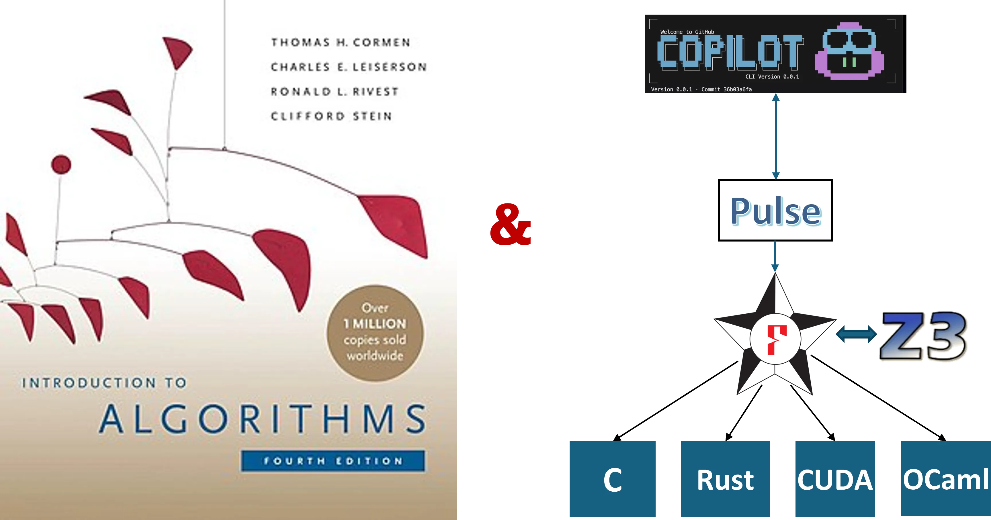
Note: Introduction to Algorithms, often referred to as CLRS, is available from MIT Press. The image above uses Wikipedia’s cover image for the book, which is available under a fair-use policy. We did not train any AI models on the content of this book, and we do not have any special access to its content. We simply used a PDF of the book, converted to text by pdftotext, and allowed agents to reference this content when implementing and proving the algorithms.

The ability to produce provably correct code at this scale is, frankly, jaw dropping. But, many challenges remain, with the most prominent being “how to effectively audit specifications?“. This post highlights some interesting examples from this experience, but let’s start with a few main takeaways.

• Program Proof Tools Work!

  Tools to formally prove the correctness of programs, including low-level imperative programs, have been around for a while and are quite capable of handling proofs of non-trivial algorithms and data structures. That said, the expressiveness of program logics is important and Pulse’s concurrent separation logic is naturally suited to proofs of pointer manipulating code, including things like cyclic data structures. Enhancing expressive power and proof automation remains an important research direction, enabling more program properties to be stated and checked mechanically, and reducing the manual reviewing effort.

• Specification Review is a Key Challenge

  Proofs are great, but only as good as the properties they establish. Even with provably correct code, AI slop is real, especially in that it can prove specifications that are not necessarily what one would want, both in terms of the properties themselves and in terms of abstraction and reuse. However, with multiple rounds of specification critique and revision, it is possible to get agents to produce good specifications. Easing the process of specification audit, and matching those against intent, is perhaps the most important open problem in this space. Shuvendu Lahiri’s recent post on intent formalization is right on the mark here.

• Empirical Language Design and Usability Studies

  With agents pounding away at our programming tools, we have a great opportunity to conduct empirical PL usability and design studies, mining traces of agent logs to understand where the tools work well and where the agents workaround rough edges. At a more conceptual level, one could also study different agentic programming and proof strategies, efforts that have only recently started to be explored, with much difficulty, on small groups of human programmers (e.g., see this recent paper). Improving tools for both human and agentic use is an important direction to pursue.

• AutoCLRS is Available, Though Still a Work in Progress

  Our agent-generated code and proofs are available at FStarLang/AutoCLRS. By no means is this is a complete formalization of the book, and it is far from polished. But, it is a substantial start, and we plan to keep improving it, with a few possible eventual goals.

  • We believe this could serve as a useful reference guide for future uses of F* and Pulse, both human and agentic. Already, in several other projects, agents have referenced this code to understand how to write certain kinds of proofs, and we expect, with (much more) further polish, this could become more useful still. Parts of it will also eventually be included in the F* and Pulse standard library.

  • Again, with more work, we believe it could be possible to extract the code into standalone, reusable libraries in OCaml, C, or Rust, usable by others beyond the F* and Pulse community. This could serve as a repository of high-assurance algorithms and data structures for general-purpose usage.

  • We welcome any feedback and contributions to the repository, especially in terms of specification review---there’s a lot of work still left to do!

Setup

If you’re unfamiliar with F* and Pulse, see my previous post for some quick background.

As in my previous post, we used Copilot CLI, this time with Opus 4.6, using Copilot CLI’s autopilot mode. One has to use this with care, since the agent has full access to the machine---I used a relatively locked-down machine whose state I didn’t care much about. That said, I also did not observe the agent doing anything nefarious.

Unlike previously, this time I also wired up FStar-MCP, a tool that Lef built on top of the LSP server FStar-VSCode-Assistant. This allows the agent to interact incrementally with the F* type checker in multiple concurrent sessions, with the server maintaining state to track which parts of a file have already been checked. This improves the latency of checking agent output, and since these proofs take many iterations of verifier feedback, reducing the latency helps keep things moving. However, I also found that agents don’t always use the MCP server and fallback to just running F* from the command line.

The agent had access to a PDF of CLRS. My initial prompt was just a single line “pick a collection of algorithms and data structures from CLRS to implement with proofs of functional correctness in F* and Pulse”. It picked around 50 algorithms and data structures spread across 22 chapters. Some of the chapters it left out did not have any algorithms in them---they instead provide mathematical background. Other chapters on randomized algorithms and multi-threaded algorithms were also left out---these could be interesting to look into for the future, since especially the multi-threaded algorithms would be a great fit for Pulse’s concurrent separation logic.

The agent produced around 10,000 lines of code and proofs very quickly, but my initial excitement quickly turned to the question of how to review what was proven. It took about a month of nudging the process, a relatively hands-off interaction while I was doing other things, to reach this point---100,000 lines of code and proofs, with a very rough count of around 5,000 lines of specification to be audited. That’s a big chunk of specification to review, and reviewing each of them also requires understanding the corresponding algorithm from CLRS, but it’s significantly less than the total amount of code and proofs. That’s one of the main advantages of proof-oriented programs: the proofs are checked mechanically, so one only has to review the specifications.

The Catalog

Here’s a catalog of what was developed: 52 algorithms and data structures, with functional correctness proofs and many with some complexity results. That said, take this table with a big grain of salt---it was produced by an AI review of the entire development. As we look at some of the examples in detail, you’ll see that while the proofs are all mechanically checked, the quality of specification and exactly what is proven is highly variable. We’ve started the process of reviewing all these specifications in detail, first using several rounds of AI-based review, but ultimately this will require a detailed human expert review. If you want to contribute, or have ideas for how to make review easier, we’d love to hear from you.

Legend:

• Spec = what the postcondition proves
• Complexity = “Linked” if ghost counters are threaded through the Pulse implementation; “Pure” if proven separately in F*; ”—” if none

#	Algorithm	CLRS	Spec	Complexity
1	Insertion Sort	§2.1	sorted ∧ permutation	Linked O(n²)
2	Merge Sort	§2.3	sorted ∧ permutation	Linked O(n lg n)
3	Binary Search	§2.3	found ⟺ key in array	Linked O(lg n)
4	Kadane (Max Subarray)	§4.1	result = max contiguous sum	Linked O(n)
5	D&C Max Subarray	§4.1	result = max contiguous sum	Pure O(n lg n)
6	Matrix Multiply	§4.2	C = A · B	Linked O(n³)
7	Strassen	§4.2	Strassen = standard mult	Pure O(n^{2.81})
8	Heapsort	§6.4	sorted ∧ permutation	Linked O(n lg n)
9	Partition	§7.1	elements partitioned ∧ perm	Linked Θ(n)
10	Quicksort	§7.1	sorted ∧ permutation	Linked O(n²)
11	Counting Sort	§8.2	sorted ∧ permutation	—
12	Counting Sort (Stable)	§8.2	stable sort ∧ perm	—
13	Radix Sort	§8.3	sorted ∧ permutation	—
14	Bucket Sort	§8.4	sorted ∧ permutation	—
15	Min / Max	§9.1	result ∈ array ∧ is min/max	Linked Θ(n−1)
16	Simultaneous Min-Max	§9.1	min ∧ max of array	Linked ⌊3(n−1)/2⌋
17	Quickselect	§9.2	k-th smallest at position k	Linked O(n²)
18	Partial Selection Sort	§9.2	first k sorted, k-th correct	Linked O(nk)
19	Stack	§10.1	ghost list matches (LIFO)	—
20	Queue	§10.1	ghost list matches (FIFO)	—
21	Singly Linked List	§10.2	ghost list matches contents	Linked O(n)
22	Doubly-Linked List	§10.2	segment pred ∧ ghost list	—
23	Hash Table (Linear Probing)	§11.4	key ↦ value lookup	—
24	BST (Pointer-based)	§12.1–3	key set ∧ BST invariant	Linked O(h)
25	BST (Array-based)	§12.1–3	key set ∧ BST invariant	Linked O(h)
26	RB Tree (Okasaki)	§13.1–4	BST ∧ RB invariants	Pure O(lg n)
27	RB Tree (CLRS-style)	§13.1–4	BST ∧ RB invariants + delete	—
28	Rod Cutting	§15.1	optimal revenue	Linked O(n²)
29	LCS	§15.4	LCS length	Linked O(mn)
30	Matrix Chain	§15.2	optimal parenthesization cost	Pure O(n³)
31	Activity Selection	§16.1	greedy = optimal count	Linked O(n)
32	Huffman Coding	§16.3	WPL-optimal prefix-free tree	Pure O(n²)
33	Union-Find	§21.3	find/union maintain forest	—
34	BFS	§22.2	distances ∧ parent tree	Linked O(V²)
35	DFS	§22.3	timestamps ∧ classification	Linked O(V²)
36	Kahn Topological Sort	§22.4	valid topological order	Linked O(V²)
37	Kruskal MST	§23.2	forest of graph	Pure O(V³)
38	Prim MST	§23.2	spanning tree + key correct	Pure O(V²)
39	MST Theory	§23.1	cut/cycle properties	—
40	Bellman-Ford	§24.1	SSSP distances	Linked O(V³)
41	Dijkstra	§24.3	SSSP distances	Linked O(V²)
42	Floyd-Warshall	§25.2	APSP distances	Linked Θ(n³)
43	Edmonds-Karp (Max Flow)	§26.2	valid flow ∧ max flow	Pure O(VE²)
44	GCD / Extended GCD	§31.2	gcd ∧ Bézout coefficients	Linked O(lg b)
45	Modular Exponentiation	§31.6	result = b^e mod m	Linked O(lg e)
46	Naive String Match	§32.1	all match positions	Linked O(nm)
47	KMP	§32.4	all match positions	Linked O(n+m)
48	Rabin-Karp	§32.2	all match positions	Pure O(nm)
49	Segments (Primitives)	§33.1	correct intersection test	—
50	Graham Scan	§33.3	convex hull (all left turns)	—
51	Jarvis March	§33.3	convex hull vertices	—
52	Vertex Cover (2-approx)	§35.1	cover ≤ 2 · OPT	—

I should also say, as pointed out in my previous post, that specifications are not absolute. There are aspects of program behavior that one still has to check manually. Performance properties are a good example of this, but in the case of AutoCLRS, one also has to check if the algorithm implemented is really the one that was intended, e.g., is an implementation that claims to be Quicksort really implementing the Quicksort algorithm and not actually implementing, say, insertion sort. Or, more subtly, does it implement Hoare’s partition algorithm or Lomuto’s, as Tahina observed.

Dijkstra’s Shortest Path Algorithm

Dijkstra’s classic shortest-path algorithm is described in Chapter 24 of CLRS. Here’s the top-level signature of what is proven about it in AutoCLRS: this is quite a lot to digest, so we’ll describe it in detail below.

fn dijkstra
  (weights: A.array int)
  (n: SZ.t)
  (source: SZ.t)
  (dist: A.array int)
  (pred: A.array SZ.t)
  (ctr: GR.ref nat)
  requires
    A.pts_to weights sweights **
    A.pts_to dist sdist **
    A.pts_to pred spred **
    GR.pts_to ctr c0 **
    pure (
      SZ.v n > 0 /\
      SZ.v source < SZ.v n /\
      Seq.length sweights == SZ.v n * SZ.v n /\
      Seq.length sdist == SZ.v n /\
      Seq.length spred == SZ.v n /\
      SZ.fits (SZ.v n * SZ.v n) /\
      all_weights_non_negative sweights /\
      weights_in_range sweights (SZ.v n)
    )
  ensures exists* sdist' spred' (cf: nat).
    A.pts_to weights sweights **
    A.pts_to dist sdist' **
    A.pts_to pred spred' **
    GR.pts_to ctr cf **
    pure (
      Seq.length sdist' == SZ.v n /\
      (forall (v: nat). v < SZ.v n ==>
        Seq.index sdist' v == SP.sp_dist sweights (SZ.v n) (SZ.v source) v) /\
      shortest_path_tree spred' sweights (SZ.v n) (SZ.v source) /\
      dijkstra_complexity_bounded cf (reveal c0) (SZ.v n)
    )

• The weights array represents the weights of edges in a graph with n vertices, represented as a flattened n * n array. The contents of the weights array is the logical variable, sweights. The source vertex is represented as an index into the array. Array indices and sizes in Pulse are represented using the type SZ.t (analogous to size_t in C).

• dist and pred are out parameters. dist will be filled with the shortest path distances from the source to each vertex, and pred will be filled with the predecessor of each vertex in the shortest path tree rooted at source.

• ctr is a ghost counter which is used to count “ticks”, the number of steps to be accounted for when computing worst-case complexity bounds for the algorithm---exactly which operations are counted as “ticks” is part of the specification, something we’ll describe in more detail below. The initial value of the ctr is c0.

Aside from constraints on the dimensions of all the arguments, the main preconditions include the following:

• All the weights in the graph must be non-negative: this is an important precondition for Dijkstra’s algorithm to work correctly.

• The second precondition is a technicality: the weights are represented as integers, which in F* are unbounded mathematical integers (implemented using a bignum library). CLRS’s describes the algorithm by setting the shortest paths of all vertices to infinity at the start and then updating those values as the algorithm proceeds. The int type in F* does not have an infinity value, so the precondition weights_in_range says that all weights must be bounded, so that the algorithm can pick a sufficiently high value and designate it as the placeholder value for a still to be computed path.

Now for the postcondition, or the ensures clause:

• The weights array is unchanged, but the dist and pred arrays are updated to sdist' and spred', which are the logical variables representing the contents of those arrays.

• For all vertices, the value in sdist' at that vertex is equal to the shortest path
  distance from the source to that vertex, as computed by a pure function SP.sp_dist.

• The pred array represents the shortest path tree rooted at source, as expressed by the predicate shortest_path_tree.

• And the final value of the tick counter ctr is cf, and it is related to c0 by dijkstra_complexity_bounded.

To judge if this is actually a useful specification, one now has to review all the auxiliary predicates used here, i.e., sp_dist, shortest_path_tree, and dijkstra_complexity_bounded.

Proofs by Functional Refinement: SP.sp_dist

A common style in formalizing imperative algorithms and data structures is to first write a purely functional specification of the algorithm or data structure, and then to prove that the imperative implementation refines the functional specification. Separately, one can then prove that the functional specification satisfies the properties that one wants. This is also the style used in AutoCLRS, with the SP.sp_dist postcondition of Dijkstra being a good example.

SP.sp_dist is a recursive, pure function computing the shortest path from s to v in the weighted graph represented by weights and n.

let sp_dist (weights: Seq.seq int) (n: nat) (s v: nat) : int = ...

Its precise definition is not that important, because the agent proves the following properties about it:

• First, that the sp_dist weight of a path is less than or equal to the weight of any other path from s to v. Of course, now one also has to check that path_weight etc. are meaningfully defined.

let sp_dist_optimal (weights: Seq.seq int) (n: nat) (s v: nat) (p: path)
  : Lemma
    (requires n > 0 /\ s < n /\ v < n /\ Seq.length weights == n * n /\
              path_source p == s /\ path_dest p == v /\
              path_edges p <= n - 1 /\
              path_valid p n /\ path_all_edges_exist p weights n /\
              all_weights_non_negative weights)
    (ensures sp_dist weights n s v <= path_weight p weights n)

• Second, that a path with the sp_dist actually exists, proven using the pure function below that computes a path whose weight is exactly the sp_dist.

let sp_dist_achievable  (weights: Seq.seq int) (n: nat) (s v: nat)
  : Pure path
    (requires n > 0 /\ s < n /\ v < n /\ Seq.length weights == n * n /\
              sp_dist weights n s v < inf)
    (ensures fun p ->
      path_source p == s /\ path_dest p == v /\
      path_edges p <= n - 1 /\
      path_valid p n /\ path_all_edges_exist p weights n /\
      path_weight p weights n == sp_dist weights n s v) = ...

shortest_path_tree

Here is the the definition of shortest_path_tree:

let shortest_path_tree (spred: Seq.seq SZ.t) (sweights: Seq.seq int) (n source: nat) : prop =
  Seq.length spred == n /\
  Seq.length sweights >= n * n /\
  source < n /\
  SZ.v (Seq.index spred source) == source /\
  (forall (v: nat). v < n /\ v <> source /\ SP.sp_dist sweights n source v < SP.inf ==>
    (let p = SZ.v (Seq.index spred v) in
     p < n /\
     SP.sp_dist sweights n source v ==
       SP.sp_dist sweights n source p + Seq.index sweights (p * n + v)))

Focusing on the most important parts, this says:

• The predecessor of the source vertex is itself, which is a common convention for shortest path trees.

• For any other vertex v, if the SP.sp_dist for that vertex is not the placeholder value, then there is a valid predecessor p for that vertex, and the SP.sp_dist for v is equal to the SP.sp_dist for p plus the weight of the edge from p to v.

This specification looks good, but it is a little ugly---note the use of p * n + v to index into the flattened weights array. A more abstract representation of the weights matrix in the specification would be easier to use and review.

Finally, we have one more property to prove, i.e., when the sp_dist of a vertex is SP.inf, then it is unreachable from the source. That’s also proven, below:

val sp_dist_inf_means_unreachable (sweights: Seq.seq int) (n source v: nat)
  : Lemma
    (requires
      weights_in_range sweights n /\
      n > 0 /\ source < n /\ v < n /\
      Seq.length sweights == n * n /\
      all_weights_non_negative sweights /\
      SP.sp_dist sweights n source v == SP.inf)
    (ensures ~(SP.reachable sweights n source v))

Of course, one must also review the definition of SP.reachable: I’ll spare you the details here, but it is defined, as expected, in terms of an existence of a path from source to v.

Complexity bounds: dijkstra_complexity_bounded

A standard technique for proving complexity bounds for implementations of algorithms is to instrument the code with “ticks” to count relevant operations. For example, Danielsson’s paper from POPL 2008 uses this technique.

The agents initially focused on the functional correctness proofs only. I instructed it to also formalize complexity results by instrumenting the code with a ghost counter (ghost values exist only for specification & proof and cannot influence the runtime behavior of a program), explicitly counting ticks by incrementing the counter, and then writing invariants and proofs to bound the total number of ticks.

Here’s the complexity result for Dijkstra’s algorithm, i.e., the total number of iterations is O(n^2), which is what one would expect for the adjacency matrix representation chosen here.

let dijkstra_iterations (n: nat) : nat = n + 2 * n * n

let dijkstra_complexity_bounded (cf c0 n: nat) : prop =
  cf >= c0 /\ cf - c0 == dijkstra_iterations n

Of course, now one also has to audit exactly which operations were counted as ticks. A manual inspection of the code shows:

• A tick for each iteration of the initialization loop, setting the initial distances to the placeholder SP.inf value.

• A tick counted for each iteration of find_min_unvisited, a helper function to find the minimum distance unvisited vertex.

• A tick for each iteration of the inner edge relaxation loop.

Again, a bit of ugliness: Guido points out that cf >= c0 is redundant, since dijkstra_iterations n is non-negative anyway.

Termination Proofs: Agents Pickup New Features

In my previous post, I mentioned that although all pure functions in F* are proven terminating, proofs of Pulse program proofs were limited only to provide partial correctness results, i.e., a Pulse program may loop forever, but if it returns, it satisifies its postcondition. This is a common limitation in many concurrent separation logics, and indeed, in the most general case (e.g., to represent processes that may intentionally run forever), one cannot prove termination, aiming instead for other properties, e.g., liveness.

However, for the sequential algorithms considered in AutoCLRS, it is possible to prove termination relatively easily, by reusing F*‘s support for well-founded orders to also check the termination of loops in Pulse. In the process of doing this work, we realized that not checking termination of this code was a significant limitation and made the task of reviewing the code so much harder. So, Gabriel quickly whipped up support for a new feature in Pulse, adding decreases clauses as a termination measure for while loops, and getting the Pulse checker to actually prove that this measure decreases at each iteration.

With this new feature in place, and a few handwritten examples showing how to use it in the Pulse library, the model quickly picked up the idea and proceeded to add decreases measures to nearly all the while loops in the library. So, the agent’s implementation of Dijkstra’s algorithm is also proven totally correct, i.e., it terminates with the correct result on all inputs.

Many Iterations to a Proven Implementation

As you can see from just this example, judging the quality of a proven implementation is a non-trivial process and requires a careful reading and also some knowledge of the proof techniques that are involved. I’ve shown you the final version of the code, but it took many iterations to get there. There have been more than 600 commits to the AutoCLRS repository so far, and the commit history shows how the code and proofs evolved.

For Dijkstra’s algorithm and related modules alone, there are 46 commits, with each commit itself involving hundreds of code edits and invocations of the compiler tools, and countless other tool invocations (e.g., bash, sed, grep commands to search libraries, monitor processes etc.). I provided specific feedback on the specifications of Dijkstra’s algorithm roughly a dozen times, usually a couple of times a day, when I had time to check on the agents’ progress. Let me quickly cover a few prior versions to illustrate the path:

Initial version: Almost trivial

This first version had an extremely weak specification, mainly just proving that in the output dist array, the distance from the source vertex to itself is less than or equal to 0, a laughably weak specification.

  ensures exists* sdist'.
    A.pts_to weights sweights **
    A.pts_to dist sdist' **
    pure (
      Seq.length sdist' == SZ.v n /\
      (SZ.v source < Seq.length sdist' ==> Seq.index sdist' (SZ.v source) <= 0)
    )

Intermediate versions with strange runtime checks

As I instructed the agent to strengthen specifications, things started to get better, but the intermediate versions had all kinds of other problems. For example, this was one version:

fn dijkstra ... (tri_result: R.ref bool)
requires ...
ensures ...
    R.pts_to tri_result vtri **
    pure ( ...
     (vtri == true ==> triangle_inequality sweights sdist' (SZ.v n)))

This version took an extra out parameter tri_result and the code had a strange extra loop at the end of the algorithm checking to see if the triangle inequality holds for the computed distances, and setting tri_result to true if it does. This is obviously wrong, and surprising, since surely the model’s background knowledge about Dijkstra’s algorithm is very strong. My hunch was that it was trying to mimic a check at the end of Bellman-Ford’s algorithm (also in the same chapter), which does have a check for negative weight cycles at the end, and it got confused and added a similar check to Dijkstra’s algorithm.

I had several rounds of agents reviewing specifications to spot gaps and mistakes, but those agents failed to spot this gaffe, and it fell to me to notice it.

Partial specifications

As things progressed, specifications got stronger, but there were still gaps. For example, in one version, the specification included the following, which shows that the computed distances are upper bounded by SP.sp_dist, which is not sufficient, since one could also satisfy this just by filling sdist' with zeroes.

  ensures ...
    (forall (v: nat). v < SZ.v n ==>
      Seq.index sdist' v <= SP.sp_dist sweights (SZ.v n) (SZ.v source) v) /\

Trivial Complexity Proofs

As the agent started to add complexity proofs, some of the initial versions were trivial, e.g., rather than counting operations with individual ticks, the agent would simply update the tick counter with a large number at the end of the algorithm, which is not a useful proof at all.

After a few iterations, the tick increments chosen by the agent (described above) seemed reasonable. Note that these ticks only account for this algorithm, treating every call to the standard library as zero-cost. Enforcing proper ticking conventions by wrapping all the basic Pulse libraries (for arrays, references etc.) with ticks would ensure that the model would have to account for all ticks. Though, this would also pollute the libraries with tick accounting, not usually something one does in real systems implementations.

Functional Specifications vs Declarative Specifications

Many times, the agent produces a proof that the imperative Pulse code refines a purely functional algorithm. For example, in Dijkstra’s algorithm, we had SP.sp_dist as our functional reference algorithm. But, this refinement proof alone is usually a proof device, and not the final result. Showing that the functional specification actually computes the correct result is also very important, e.g., lemmas such as sp_dist_optimal and sp_dist_achievable above are crucial to really finish the proof.

Some Takeaways

All of this should make it clear that the agents do not magically produce exactly the right specification on the first try. Reviewing the specifications and instructing the agents to strengthen them to arrive at what one wants is a crucual part of the process.

In this work, I chose to go bottom-up: have the agents implement a whole bunch of algorithms and then critique the specs and iterate with the agents until we arrived at specifications we wanted. In hindsight, it might have been better to also go top-down, i.e., start by iterating with the agents to write down the desired specifications for all the algorithms, and once the specifications were settled, unleash the agents to implement the code and write all the proofs.

The breadth-wise scale of this work was also a challenge: needing to understand and review 50 different algorithms and data structures, each with their own specifications and proof techniques, made it hard to keep track of all the details. Proceeding depth-first on one algorithm at a time may have also been easier to review and to get right, though it may have taken more time to reach the current scale.

Take this also a disclaimer about the entire library: many parts of it are in various stages of the specification review & agent revision process. You can see some interesting interactions between human reviewers writing issues and agents responding with comments and commits to address them in the AutoCLRS repository, e.g., (issue 2, issue 3, issue 4). Understanding how to evolve this process into a scalable human-agent collaboration process for specification review and revision is an interesting open question, one that we have started to think about.

Parting Thoughts

It’s been a fascinating journey to see how agents can develop a large corpus of verified code and proofs with only natural language guidance, both from textbook descriptions and from specification review by a human. My impression is that agents have mastered the mechanics of low-level proof engineering, at least for program proofs of the kind needed for CLRS, but need a lot of guidance on high-level proof and specification architecture.

Program Logics Forever

One might be tempted to think that proof engineering is now totally automated and that research in program logics and proof techniques is no longer needed---I don’t think this is the case at all, from several dimensions.

First, techniques that enable greater abstraction and modularity will lead to more fluent proofs for agents as well as for humans. To pick just one concrete example, a prior program logic in F* called Low* supported proofs of pointer-manipulating data structures. However, proofs in Low* are painfully non-modular, requiring reasoning about the entire heap at each step, so much so that even proofs of canonical data structures like doubly linked lists in Low*, took a PhD student many painful months to implement---getting an agent to do the same in Low* would also be a struggle. In contrast, agents were able to easily develop a Reynolds-style formalization of doubly linked lists in Pulse pretty quickly.

Second, expanding the expressiveness of program logics to allow more kinds of properties to be stated and checked mechanically will remain an important research direction. With agents churning out code and proofs, the more we are able to check mechanically, the less there is to review manually, and reviewing seems to now be the main bottleneck. We already have a small example of this: our addition of termination proof checking in Pulse was an expressiveness boost, and resulted in a corresponding reduction in reviewing effort.

Finally, although it appears that models use Turing complete programming languages and general purpose program logics effectively, I believe domain-specific languages and tools to automate high-assurance coding will continue to be important. For instance, rather than having an agent write a low-level parser directly in C and then trying to prove it secure, agents should be able to author high-level grammars and use verified parser generators (e.g., EverParse) to get the job done. Not only will this be easier for humans and other agents to review, but it will also avoid costly model invocations to add proofs to large amounts of low-level code---why bother with that when correct-by-construction synthesis is possible?

Learning from Agents

Agents appear highly capable of coping with the rough edges of a proof assistant, and, to be honest, Pulse and F* have many. Mining agent logs to find common pitfalls and workarounds is an exciting direction for future work.

An interesting anecdote: In the process of using the newly added decreases feature, the agent noticed a limitation of the feature which caused it to fail to accept proofs in cases where the condition of the while loop had a non-trivial precondition. It also found a way to workaround the limitation and was able to provide a minimal example to illustrate the issue, which we were then able to fix.

But this is just the tip of the iceberg. Many in the programming languages community have for long aspired to study the use of PL tools in an empirical setting, but it has always been hard to do so in a controlled way and at scale. With agents driving our tools, we have an opportunity to do empirical work at scale, both learning how agents use PL tools and then learning how to improve them. That said, one has to think carefully about between improvements that cater to agents versus human users.

Finally, many of the questions and limitations I raised in my previous post, ranging from trust in verifiers to the cost of running agents at scale, remain.